Thinking of Probabilities in Terms of Areas
This note describes an approach for intuitively understanding many facts of probability used throughout this set of notes.
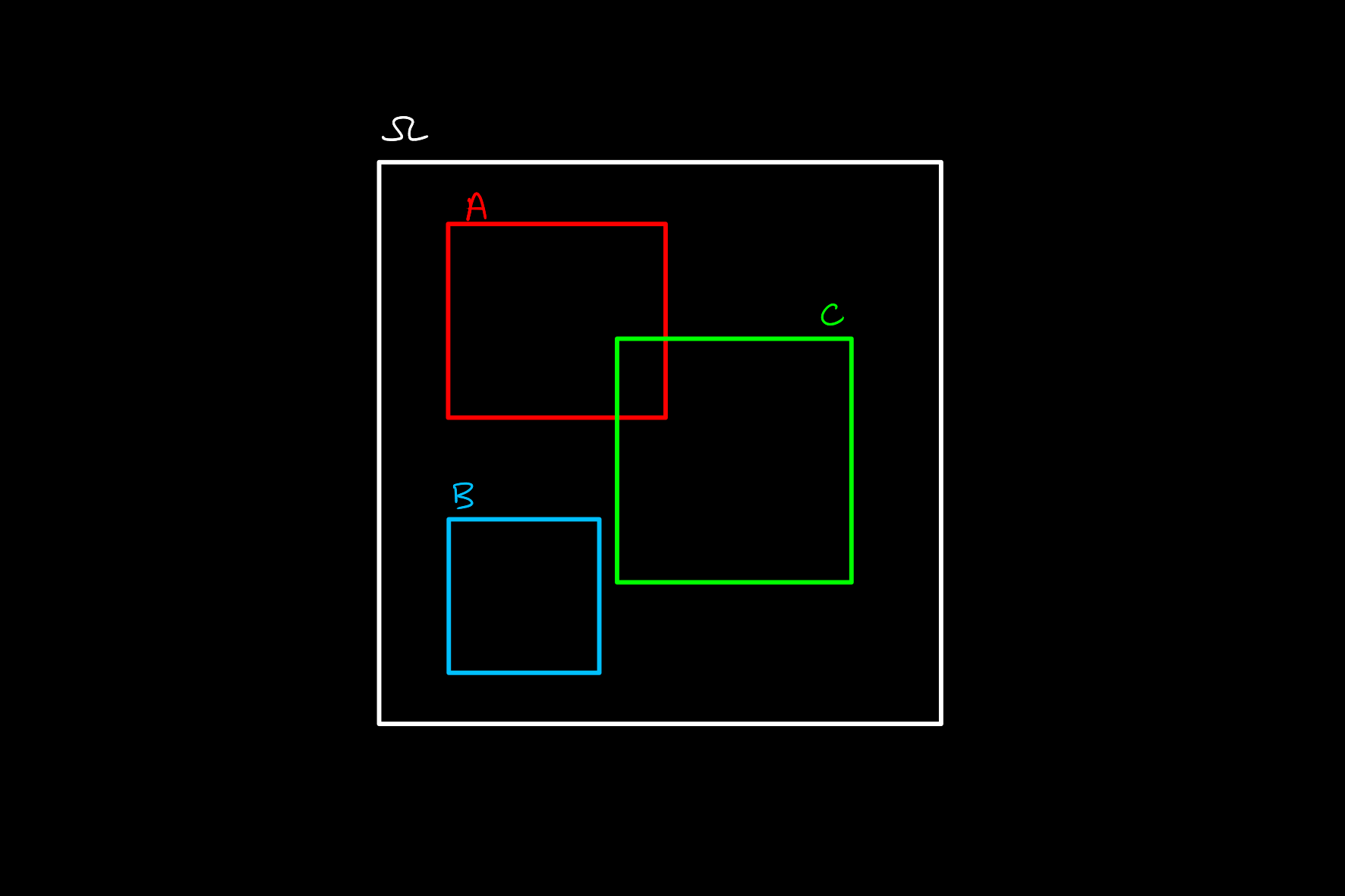
This approach is to consider the probability space

We draw this diagram such that the probability of an event occurring is equal to the area that it takes up (as a proportion of the whole area).
Then thinking of and and or conditions on probabilities in terms of the intersection and union respectively, as well as conditional probability by viewing things relative to a subset of the whole space become obvious.
It is important to note that this way of thinking about probability is not just a visual trick, or a way to obscure what is going on. Ultimately, this is just working with a particular probability space which is a subset of
Example
A classic example of a question in probability which is made significantly simpler by considering it in this way is with problems related to Bayes' theorem.
Consider the following problem:
It is known that
- Given a person is positive, they have a
- Given a person is negative, they have a
What is the probability that in individual has the disease, assuming they have tested positive?
The answer in this case (found by applying the law of total probability and bayes' theorem is
This is a result that often seems unintuitive to many people at first glance.
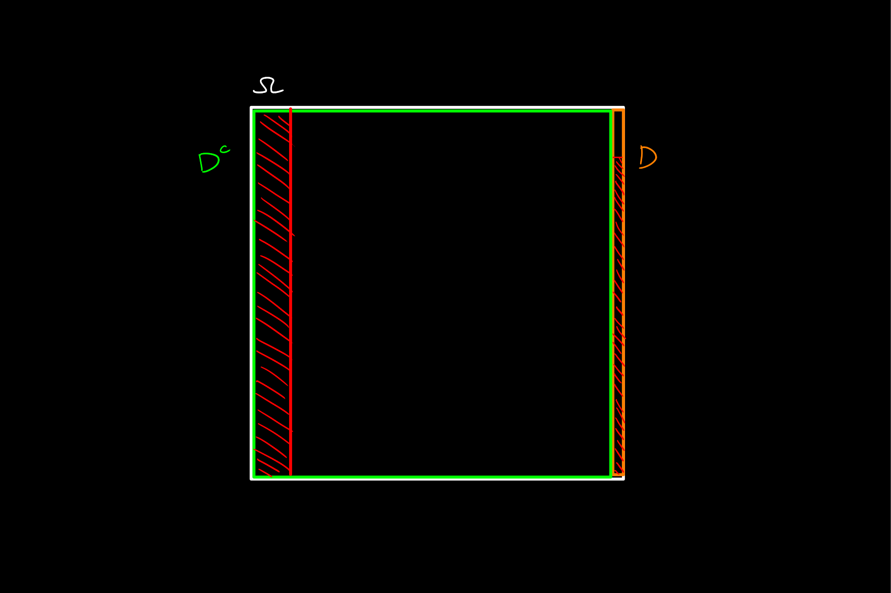
However by drawing up a probability space and representing the probabilities of events by areas, we can clearly see why this is true.
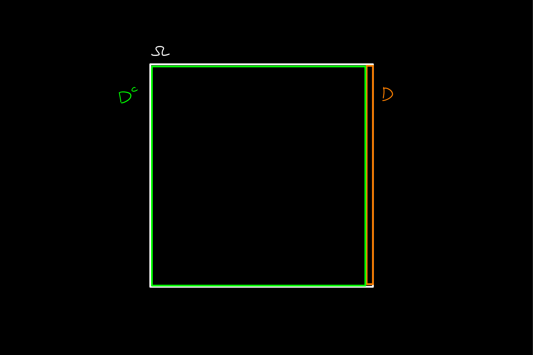
Note the below diagram where the probability of having the disease and not having the disease are shown:

And now, by colouring in the probability of a positive test in both of these cases as the corresponding proportion of each of these areas, it becomes obvious why given a positive test, it is still way more likely that you are not infected:
